Undergraduate course in Differential Equations
MATH 2552
Georgia Institute of Technology, Fall 2024

Contact: glivshyts6@math.gatech.edu; please email me with any questions (especially if the answers were not specified in the syllabus or announcements!)
TAs: Manuel Fernandez mfernandez39@gatech.edu and Tobias Wang twang740@gatech.edu.
Location and time: the class lectures meet virtually Tuesdays/Thursdays 9:30-10:45am via Zoom
August 19 through December 3, 2024.
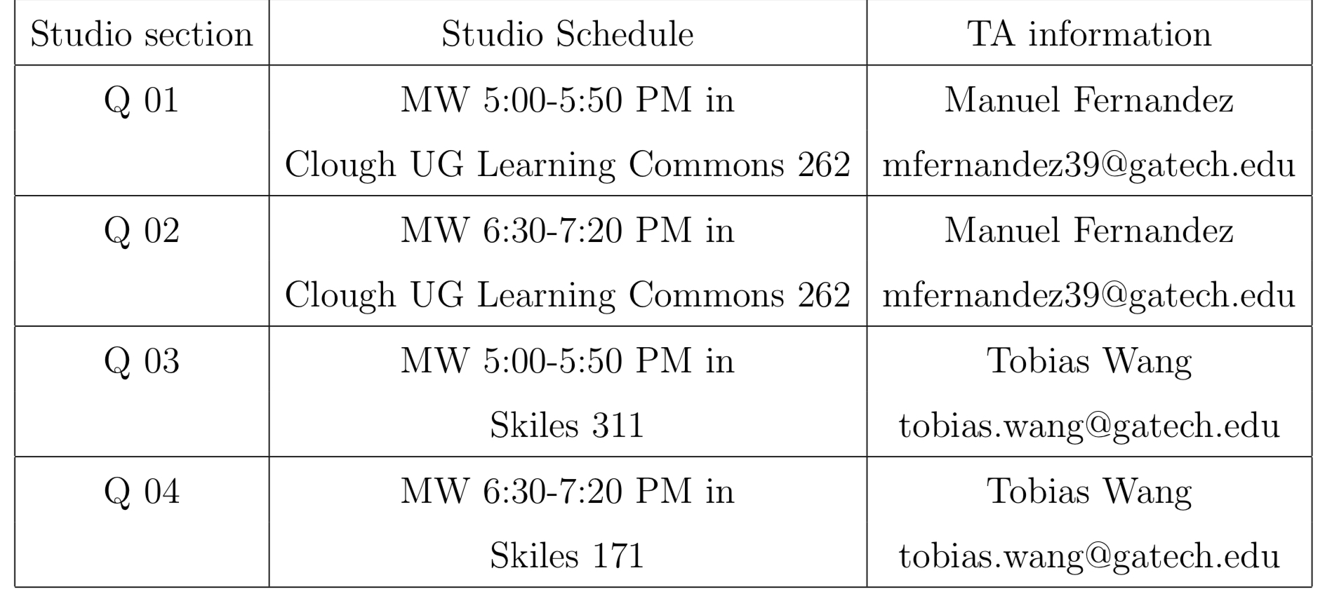
Studio times:

Office hours: Monday at 8-9:30am online via Zoom. TA office hours TBD.
Description: In this course, we cover various analytic solution methods of elementary differential equations, applications of differential equations to real world problems with modeling, qualitative studies of solutions emphasizing stability/instability. See the syllabus for more details. All the course announcements will be made via Canvas. Please make sure to follow Canvas updates. In person attendance is expected for the studios, and virtual attendance and active participation is expected for the Zoom lectures; both shall be rewarded with extra credit.
Textbook: "Differential Equations (an introduction to modern methods and applications)", James R. Brannan and William E. Boyce,3rd edition. We will cover parts of Chapters 1-8.
Homework: assigned via WebWorks weekly
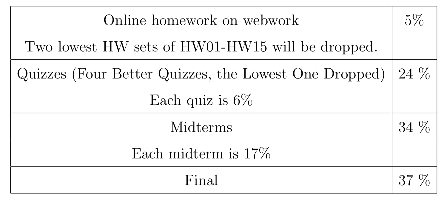
Grading:

Quizes will be held in-person during studios and the midterms and the final will take place in-person during lecture times (rooms TBA). For more details about the grading policies and extra credit opportunities, please consult the syllabus. You may view your up to date grades via Canvas or Gaderscope; the grade brackets will remain as advertised (no curving).
Class whiteboard:
Lectures 1-2:Organizational part, review of functions and derivatives, the concept of solving a differential equation, examples.
Sections 1.1, 1.2: Newton's law of cooling, solutions, initial value problem, autonomous equations, equilibrium solutions and their characterization
Lectures 3-4:Section 1.3: some summary of the definitions of differential equations, their order and a few classes, initial conditions.
Sections 2.1, 2.2: separable differential equations and the method of solving them; integral curves; linear first order differential equations and solving them using the method of integrating factors.
Section 2.3: modeling with the ODE (the example about the water container and the example about the loan).
Section 2.4, the beginning: the existence theorem for the first order linear ODE.
Lectures 5-6:Section 2.4: existence and uniqueness theorems for linear and non-linear first order differential equations; non-intersection property of solutions to these types of ODE with continuous coefficients;
Section 2.5: exponential growth model for population growth and the logistic growth equation; analyzing the solutions of the logistic equation via simple methods without solving it; more generally, analyzing solutions of autonomous equations using simple geometric methods; solving the logistic equation;
Section 2.6: exact equations and solving them by introducing an auxiliary two-variable function;
Section 2.7: substitution methods and solving homogeneous equations by substituting y=ux.
Lectures 7-10:Finishing 2.7: Bernoulli’s equations via substitution method;
3.2, 6.1, 6.2: systems of first order linear ODE — example with the greenhouse, notation and terminology, existence and uniqueness of solutions, applications to higher order ODE.
Section 3.3: relation between homogeneous and inhomogeneous systems of linear equations; superposition principle; linear independence of solutions and Wronskian; various reviews from linear algebra; how to solve a homogeneous system of linear first order ODE with fixed coefficients; some examples for two equations in the case of real different eigenvalues; trajectories and phase portraits.
3.4: complex eigenvalues; the Euler formula
3.5: homogeneous systems of 2 linear 1st order differential equations, equal eigenvalues case
shifted systems (when equilibrium exists) — starting
Lectures 11-14:Shifted systems examples (start of section 3.3 and everything done together);
Section 4.1: Second order linear ODE — examples, introduction, physical models (spring mass system, pendulum, electric circuit);
Section 4.2: existence and uniqueness of solutions; linear operators, linearity of the operators associated to second order linear equations, fundamental sets of solutions, Wronskian, Abel’s theorem about Wronskian;
Section 4.3: solving second order linear ODE with constant coefficients; characteristic quadratic equation and a complete guide to solving second order homogenous linear ODE and IVP; Cauchy-Euler equations;
Starting 4.4: undamped free vibrations.
Lectures 15-16:Finishing 4.4 — undamped free vibrations;
4.5 — homogeneous and inhomogeneous second order liner ODE; finding particular solutions via the method of varying coefficients; examples; 4.6.
Lectures 17-19:4.7 — method of variation of coefficients for systems and second order linear ODE; 5.1, 5.2 -- the concept of an integral transform, Laplace transform, several key exaples, the linearlity property, the shift property, Laplace of sin and cos, piecewise continuous functions, functions of exponential order, existence theorem, the key property that Laplace transform turns differentiation into algebraic multiplication; more properties of Laplace transform, Laplace of n-th derivative, Laplace transform turns multiplication into differentiation, Laplace of a polynomial, Laplace transform of a solution of an ODE with the IVP at 0. 5.3 Existence and uniqueness, inverse Laplace transform, table of Laplace transforms, partial fraction decomposition, examples.
The next two lectures are recordings posted ahead of time for Thursday October 31 and Tuesday November 5 correspondingly:
Lectures 20-21:5.4 -- solving ODE using Laplace transform; 5.5 -- unit step function, characteristic function, Laplace transform of such functions; periodic functions, window functions and Laplace transforms; 5.6 — ODE with discontinuous forcing functions, examples. An example of an ODE with a piecewise continuous forcing function; smoothness properties of solutions; 5.7 — delta functions and ODE with forcing functions as delta functions (modeling a hammer applied to a pendulum).
Lectures 22-23:5.8 — Convolution, properties, Laplace transform and convolution, general method of solving ODE with Laplace transforms; 7.1 — Autonomous systems, critical points/equilibria; 3 types of equilibria, the pendulum example, Section 7.2 — almost linear systems, method of linearizing, Jacobian, the pendulum example again.
Lectures 24-26:Section 7.2 continued: stability properties of equilibria of non-linear autonomous systems; 7.3 Competing species equations, examples; 7.4 predator-prey Lotka-Volterra equations; 7.6 — chaos and Lorenz equations; 8.1 -- Euler’s method of finding approximate solutions to first order ODEs.
Lecture 27, December 2:Review for the Final Exam — Q3, Q7, Q8, Q9, Q5, Q10; additional review (Thursda) Q4, Q6


